2. Over-sampling

2.1. A practical guide

You can refer to Compare over-sampling samplers.

2.1.1. Naive random over-sampling

One way to fight this issue is to generate new samples in the classes which are under-represented. The most naive strategy is to generate new samples by randomly sampling with replacement the current available samples. The RandomOverSampler offers such scheme:

>>> from sklearn.datasets import make_classification
>>> X, y = make_classification(n_samples=5000, n_features=2, n_informative=2,
...                            n_redundant=0, n_repeated=0, n_classes=3,
...                            n_clusters_per_class=1,
...                            weights=[0.01, 0.05, 0.94],
...                            class_sep=0.8, random_state=0)
>>> from imblearn.over_sampling import RandomOverSampler
>>> ros = RandomOverSampler(random_state=0)
>>> X_resampled, y_resampled = ros.fit_resample(X, y)
>>> from collections import Counter
>>> print(sorted(Counter(y_resampled).items()))
[(0, 4674), (1, 4674), (2, 4674)]

The augmented data set should be used instead of the original data set to train a classifier:

>>> from sklearn.linear_model import LogisticRegression
>>> clf = LogisticRegression()
>>> clf.fit(X_resampled, y_resampled)
LogisticRegression(...)

In the figure below, we compare the decision functions of a classifier trained using the over-sampled data set and the original data set.

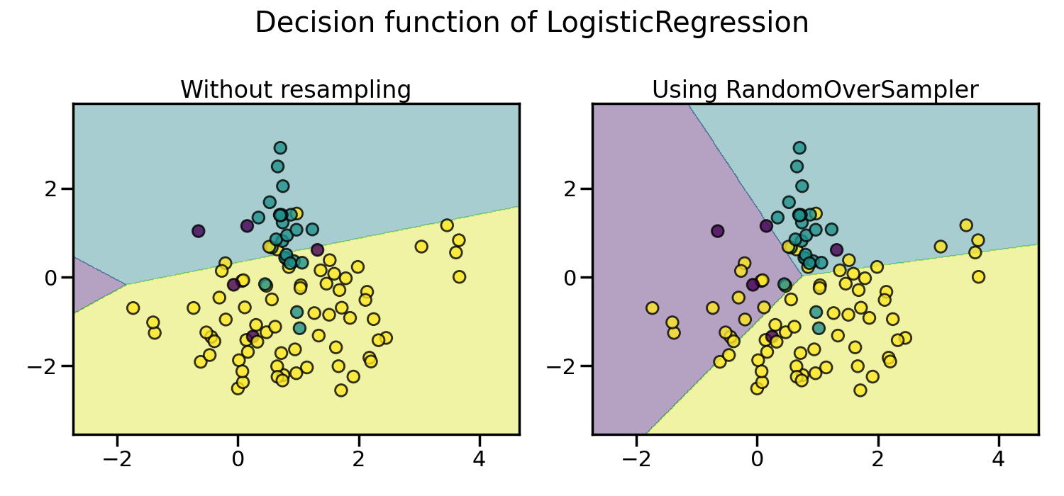
As a result, the majority class does not take over the other classes during the training process. Consequently, all classes are represented by the decision function.

In addition, RandomOverSampler allows to sample heterogeneous data (e.g. containing some strings):

>>> import numpy as np
>>> X_hetero = np.array([['xxx', 1, 1.0], ['yyy', 2, 2.0], ['zzz', 3, 3.0]],
...                     dtype=object)
>>> y_hetero = np.array([0, 0, 1])
>>> X_resampled, y_resampled = ros.fit_resample(X_hetero, y_hetero)
>>> print(X_resampled)
[['xxx' 1 1.0]
 ['yyy' 2 2.0]
 ['zzz' 3 3.0]
 ['zzz' 3 3.0]]
>>> print(y_resampled)
[0 0 1 1]

It would also work with pandas dataframe:

>>> from sklearn.datasets import fetch_openml
>>> df_adult, y_adult = fetch_openml(
...     'adult', version=2, as_frame=True, return_X_y=True)
>>> df_adult.head()  
>>> df_resampled, y_resampled = ros.fit_resample(df_adult, y_adult)
>>> df_resampled.head()  

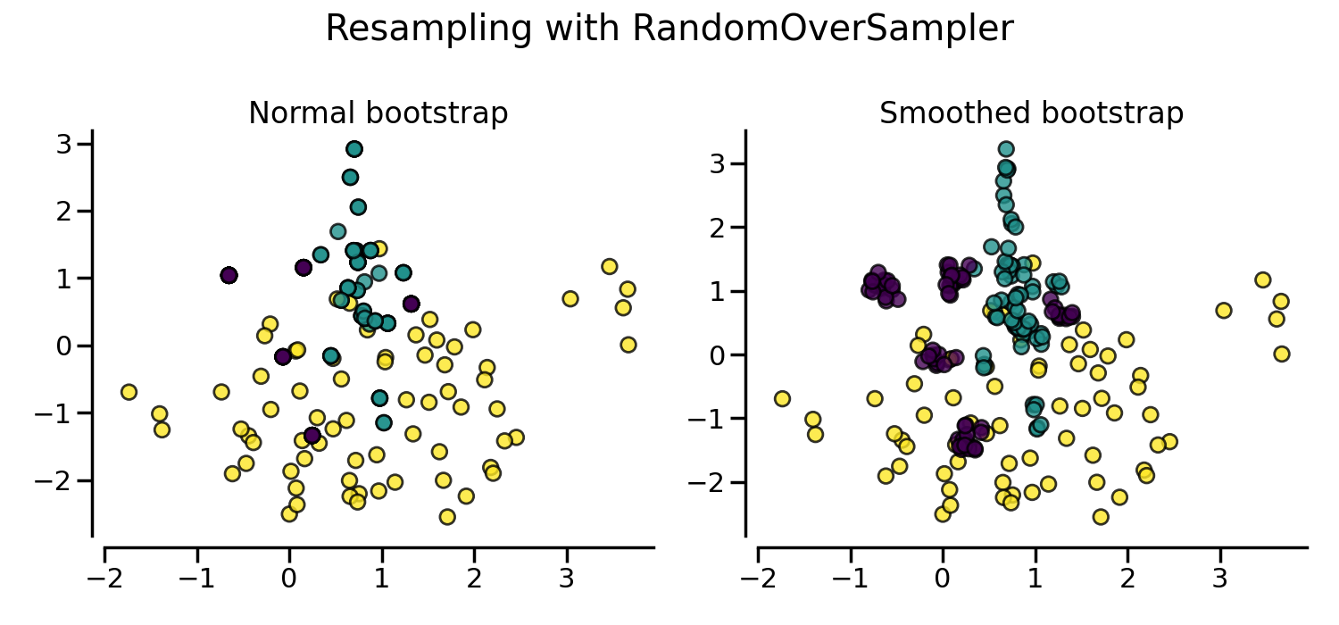
If repeating samples is an issue, the parameter shrinkage allows to create a smoothed bootstrap. However, the original data needs to be numerical. The shrinkage parameter controls the dispersion of the new generated samples. We show an example illustrate that the new samples are not overlapping anymore once using a smoothed bootstrap. This ways of generating smoothed bootstrap is also known a Random Over-Sampling Examples (ROSE) [MT14].

2.1.2. From random over-sampling to SMOTE and ADASYN

Apart from the random sampling with replacement, there are two popular methods to over-sample minority classes: (i) the Synthetic Minority Oversampling Technique (SMOTE) [CBHK02] and (ii) the Adaptive Synthetic (ADASYN) [HBGL08] sampling method. These algorithms can be used in the same manner:

>>> from imblearn.over_sampling import SMOTE, ADASYN
>>> X_resampled, y_resampled = SMOTE().fit_resample(X, y)
>>> print(sorted(Counter(y_resampled).items()))
[(0, 4674), (1, 4674), (2, 4674)]
>>> clf_smote = LogisticRegression().fit(X_resampled, y_resampled)
>>> X_resampled, y_resampled = ADASYN().fit_resample(X, y)
>>> print(sorted(Counter(y_resampled).items()))
[(0, 4673), (1, 4662), (2, 4674)]
>>> clf_adasyn = LogisticRegression().fit(X_resampled, y_resampled)

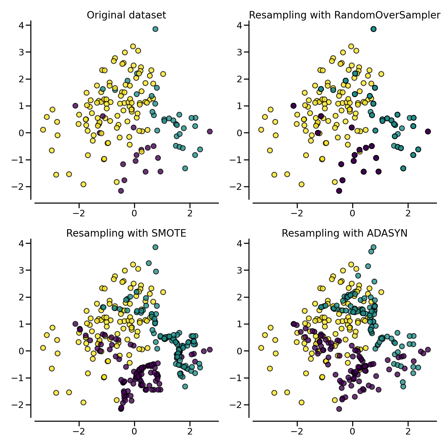
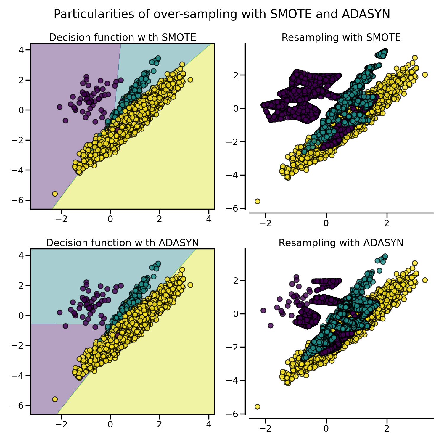
The figure below illustrates the major difference of the different over-sampling methods.

2.1.3. Ill-posed examples

While the RandomOverSampler is over-sampling by duplicating some of the original samples of the minority class, SMOTE and ADASYN generate new samples in by interpolation. However, the samples used to interpolate/generate new synthetic samples differ. In fact, ADASYN focuses on generating samples next to the original samples which are wrongly classified using a k-Nearest Neighbors classifier while the basic implementation of SMOTE will not make any distinction between easy and hard samples to be classified using the nearest neighbors rule. Therefore, the decision function found during training will be different among the algorithms.

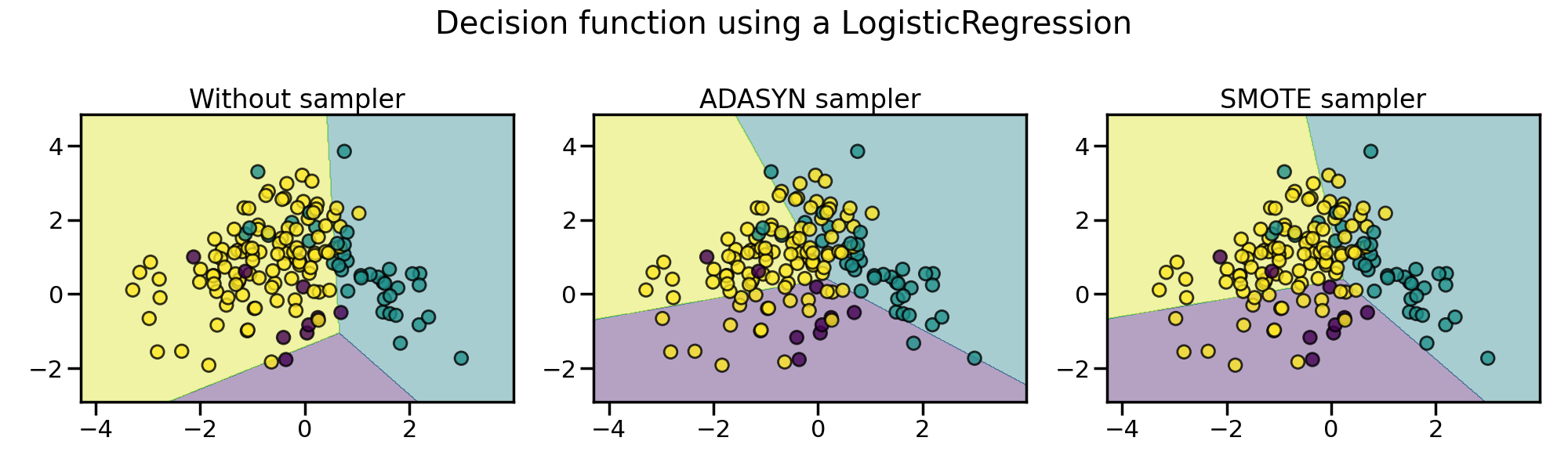
The sampling particularities of these two algorithms can lead to some peculiar behavior as shown below.

2.1.4. SMOTE variants

SMOTE might connect inliers and outliers while ADASYN might focus solely on outliers which, in both cases, might lead to a sub-optimal decision function. In this regard, SMOTE offers three additional options to generate samples. Those methods focus on samples near the border of the optimal decision function and will generate samples in the opposite direction of the nearest neighbors class. Those variants are presented in the figure below.

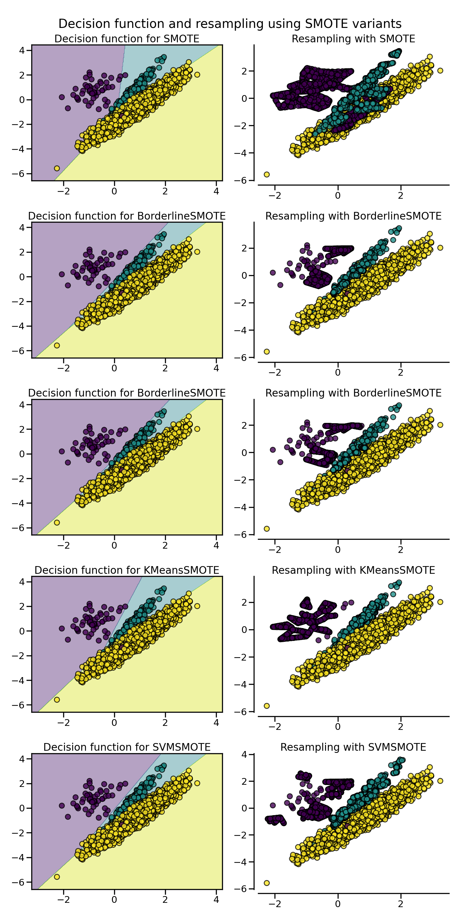
The BorderlineSMOTE [HWM05], SVMSMOTE [NCK09], and KMeansSMOTE [LDB17] offer some variant of the SMOTE algorithm:

>>> from imblearn.over_sampling import BorderlineSMOTE
>>> X_resampled, y_resampled = BorderlineSMOTE().fit_resample(X, y)
>>> print(sorted(Counter(y_resampled).items()))
[(0, 4674), (1, 4674), (2, 4674)]

When dealing with mixed data type such as continuous and categorical features, none of the presented methods (apart of the class RandomOverSampler) can deal with the categorical features. The SMOTENC [CBHK02] is an extension of the SMOTE algorithm for which categorical data are treated differently:

>>> # create a synthetic data set with continuous and categorical features
>>> rng = np.random.RandomState(42)
>>> n_samples = 50
>>> X = np.empty((n_samples, 3), dtype=object)
>>> X[:, 0] = rng.choice(['A', 'B', 'C'], size=n_samples).astype(object)
>>> X[:, 1] = rng.randn(n_samples)
>>> X[:, 2] = rng.randint(3, size=n_samples)
>>> y = np.array([0] * 20 + [1] * 30)
>>> print(sorted(Counter(y).items()))
[(0, 20), (1, 30)]

In this data set, the first and last features are considered as categorical features. One needs to provide this information to SMOTENC via the parameters categorical_features either by passing the indices, the feature names when X is a pandas DataFrame, a boolean mask marking these features, or relying on dtype inference if the columns are using the pandas.CategoricalDtype:

>>> from imblearn.over_sampling import SMOTENC
>>> smote_nc = SMOTENC(categorical_features=[0, 2], random_state=0)
>>> X_resampled, y_resampled = smote_nc.fit_resample(X, y)
>>> print(sorted(Counter(y_resampled).items()))
[(0, 30), (1, 30)]
>>> print(X_resampled[-5:])
[['A' 0.19... 2]
 ['B' -0.36... 2]
 ['B' 0.87... 2]
 ['B' 0.37... 2]
 ['B' 0.33... 2]]

Therefore, it can be seen that the samples generated in the first and last columns are belonging to the same categories originally presented without any other extra interpolation.

However, SMOTENC is only working when data is a mixed of numerical and categorical features. If data are made of only categorical data, one can use the SMOTEN variant [CBHK02]. The algorithm changes in two ways:

• the nearest neighbors search does not rely on the Euclidean distance. Indeed, the value difference metric (VDM) also implemented in the class ValueDifferenceMetric is used.

• a new sample is generated where each feature value corresponds to the most common category seen in the neighbors samples belonging to the same class.

Let’s take the following example:

>>> import numpy as np
>>> X = np.array(["green"] * 5 + ["red"] * 10 + ["blue"] * 7,
...              dtype=object).reshape(-1, 1)
>>> y = np.array(["apple"] * 5 + ["not apple"] * 3 + ["apple"] * 7 +
...              ["not apple"] * 5 + ["apple"] * 2, dtype=object)

We generate a dataset associating a color to being an apple or not an apple. We strongly associated “green” and “red” to being an apple. The minority class being “not apple”, we expect new data generated belonging to the category “blue”:

>>> from imblearn.over_sampling import SMOTEN
>>> sampler = SMOTEN(random_state=0)
>>> X_res, y_res = sampler.fit_resample(X, y)
>>> X_res[y.size:]
array([['blue'],
        ['blue'],
        ['blue'],
        ['blue'],
        ['blue'],
        ['blue']], dtype=object)
>>> y_res[y.size:]
array(['not apple', 'not apple', 'not apple', 'not apple', 'not apple',
       'not apple'], dtype=object)

2.2. Mathematical formulation

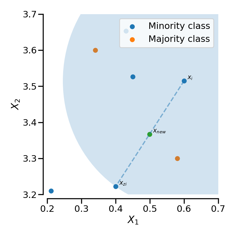
2.2.1. Sample generation

Both SMOTE and ADASYN use the same algorithm to generate new samples. Considering a sample \(x_i\), a new sample \(x_{new}\) will be generated considering its k neareast-neighbors (corresponding to k_neighbors). For instance, the 3 nearest-neighbors are included in the blue circle as illustrated in the figure below. Then, one of these nearest-neighbors \(x_{zi}\) is selected and a sample is generated as follows:

\[x_{new} = x_i + \lambda \times (x_{zi} - x_i)\]

where \(\lambda\) is a random number in the range \([0, 1]\). This interpolation will create a sample on the line between \(x_{i}\) and \(x_{zi}\) as illustrated in the image below:

SMOTE-NC slightly change the way a new sample is generated by performing something specific for the categorical features. In fact, the categories of a new generated sample are decided by picking the most frequent category of the nearest neighbors present during the generation.

Warning

Be aware that SMOTE-NC is not designed to work with only categorical data.

The other SMOTE variants and ADASYN differ from each other by selecting the samples \(x_i\) ahead of generating the new samples.

The regular SMOTE algorithm — cf. to the SMOTE object — does not impose any rule and will randomly pick-up all possible \(x_i\) available.

The borderline SMOTE — cf. to the BorderlineSMOTE with the parameters kind='borderline-1' and kind='borderline-2' — will classify each sample \(x_i\) to be (i) noise (i.e. all nearest-neighbors are from a different class than the one of \(x_i\)), (ii) in danger (i.e. at least half of the nearest neighbors are from the same class than \(x_i\), or (iii) safe (i.e. all nearest neighbors are from the same class than \(x_i\)). Borderline-1 and Borderline-2 SMOTE will use the samples in danger to generate new samples. In Borderline-1 SMOTE, \(x_{zi}\) will belong to the same class than the one of the sample \(x_i\). On the contrary, Borderline-2 SMOTE will consider \(x_{zi}\) which can be from any class.

SVM SMOTE — cf. to SVMSMOTE — uses an SVM classifier to find support vectors and generate samples considering them. Note that the C parameter of the SVM classifier allows to select more or less support vectors.

For both borderline and SVM SMOTE, a neighborhood is defined using the parameter m_neighbors to decide if a sample is in danger, safe, or noise.

KMeans SMOTE — cf. to KMeansSMOTE — uses a KMeans clustering method before to apply SMOTE. The clustering will group samples together and generate new samples depending of the cluster density.

ADASYN works similarly to the regular SMOTE. However, the number of samples generated for each \(x_i\) is proportional to the number of samples which are not from the same class than \(x_i\) in a given neighborhood. Therefore, more samples will be generated in the area that the nearest neighbor rule is not respected. The parameter m_neighbors is equivalent to k_neighbors in SMOTE.

2.2.2. Multi-class management

All algorithms can be used with multiple classes as well as binary classes classification. RandomOverSampler does not require any inter-class information during the sample generation. Therefore, each targeted class is resampled independently. In the contrary, both ADASYN and SMOTE need information regarding the neighbourhood of each sample used for sample generation. They are using a one-vs-rest approach by selecting each targeted class and computing the necessary statistics against the rest of the data set which are grouped in a single class.