Compare over-sampling samplers

The following example attends to make a qualitative comparison between the different over-sampling algorithms available in the imbalanced-learn package.

# Authors: Guillaume Lemaitre <g.lemaitre58@gmail.com>
# License: MIT

print(__doc__)

import matplotlib.pyplot as plt
import seaborn as sns

sns.set_context("poster")

The following function will be used to create toy dataset. It uses the make_classification from scikit-learn but fixing some parameters.

from sklearn.datasets import make_classification


def create_dataset(
    n_samples=1000,
    weights=(0.01, 0.01, 0.98),
    n_classes=3,
    class_sep=0.8,
    n_clusters=1,
):
    return make_classification(
        n_samples=n_samples,
        n_features=2,
        n_informative=2,
        n_redundant=0,
        n_repeated=0,
        n_classes=n_classes,
        n_clusters_per_class=n_clusters,
        weights=list(weights),
        class_sep=class_sep,
        random_state=0,
    )

The following function will be used to plot the sample space after resampling to illustrate the specificities of an algorithm.

def plot_resampling(X, y, sampler, ax, title=None):
    X_res, y_res = sampler.fit_resample(X, y)
    ax.scatter(X_res[:, 0], X_res[:, 1], c=y_res, alpha=0.8, edgecolor="k")
    if title is None:
        title = f"Resampling with {sampler.__class__.__name__}"
    ax.set_title(title)
    sns.despine(ax=ax, offset=10)

The following function will be used to plot the decision function of a classifier given some data.

import numpy as np


def plot_decision_function(X, y, clf, ax, title=None):
    plot_step = 0.02
    x_min, x_max = X[:, 0].min() - 1, X[:, 0].max() + 1
    y_min, y_max = X[:, 1].min() - 1, X[:, 1].max() + 1
    xx, yy = np.meshgrid(
        np.arange(x_min, x_max, plot_step), np.arange(y_min, y_max, plot_step)
    )

    Z = clf.predict(np.c_[xx.ravel(), yy.ravel()])
    Z = Z.reshape(xx.shape)
    ax.contourf(xx, yy, Z, alpha=0.4)
    ax.scatter(X[:, 0], X[:, 1], alpha=0.8, c=y, edgecolor="k")
    if title is not None:
        ax.set_title(title)

Illustration of the influence of the balancing ratio

We will first illustrate the influence of the balancing ratio on some toy data using a logistic regression classifier which is a linear model.

from sklearn.linear_model import LogisticRegression

clf = LogisticRegression()

We will fit and show the decision boundary model to illustrate the impact of dealing with imbalanced classes.

fig, axs = plt.subplots(nrows=2, ncols=2, figsize=(15, 12))

weights_arr = (
    (0.01, 0.01, 0.98),
    (0.01, 0.05, 0.94),
    (0.2, 0.1, 0.7),
    (0.33, 0.33, 0.33),
)
for ax, weights in zip(axs.ravel(), weights_arr):
    X, y = create_dataset(n_samples=300, weights=weights)
    clf.fit(X, y)
    plot_decision_function(X, y, clf, ax, title=f"weight={weights}")
    fig.suptitle(f"Decision function of {clf.__class__.__name__}")
fig.tight_layout()

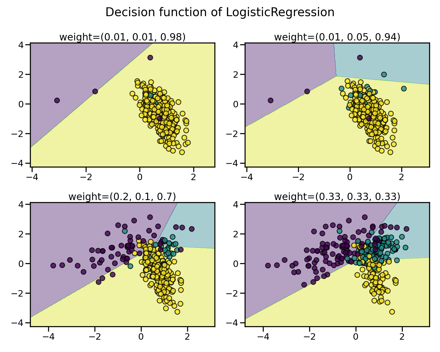
Greater is the difference between the number of samples in each class, poorer are the classification results.

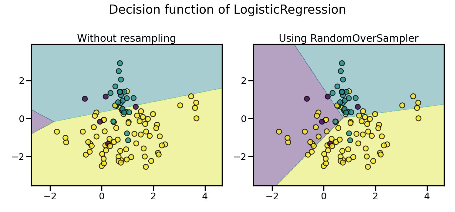
Random over-sampling to balance the data set

Random over-sampling can be used to repeat some samples and balance the number of samples between the dataset. It can be seen that with this trivial approach the boundary decision is already less biased toward the majority class. The class RandomOverSampler implements such of a strategy.

from imblearn.over_sampling import RandomOverSampler

from imblearn.pipeline import make_pipeline

X, y = create_dataset(n_samples=100, weights=(0.05, 0.25, 0.7))

fig, axs = plt.subplots(nrows=1, ncols=2, figsize=(15, 7))

clf.fit(X, y)
plot_decision_function(X, y, clf, axs[0], title="Without resampling")

sampler = RandomOverSampler(random_state=0)
model = make_pipeline(sampler, clf).fit(X, y)
plot_decision_function(X, y, model, axs[1], f"Using {model[0].__class__.__name__}")

fig.suptitle(f"Decision function of {clf.__class__.__name__}")
fig.tight_layout()

By default, random over-sampling generates a bootstrap. The parameter shrinkage allows adding a small perturbation to the generated data to generate a smoothed bootstrap instead. The plot below shows the difference between the two data generation strategies.

fig, axs = plt.subplots(nrows=1, ncols=2, figsize=(15, 7))

sampler.set_params(shrinkage=None)
plot_resampling(X, y, sampler, ax=axs[0], title="Normal bootstrap")

sampler.set_params(shrinkage=0.3)
plot_resampling(X, y, sampler, ax=axs[1], title="Smoothed bootstrap")

fig.suptitle(f"Resampling with {sampler.__class__.__name__}")
fig.tight_layout()

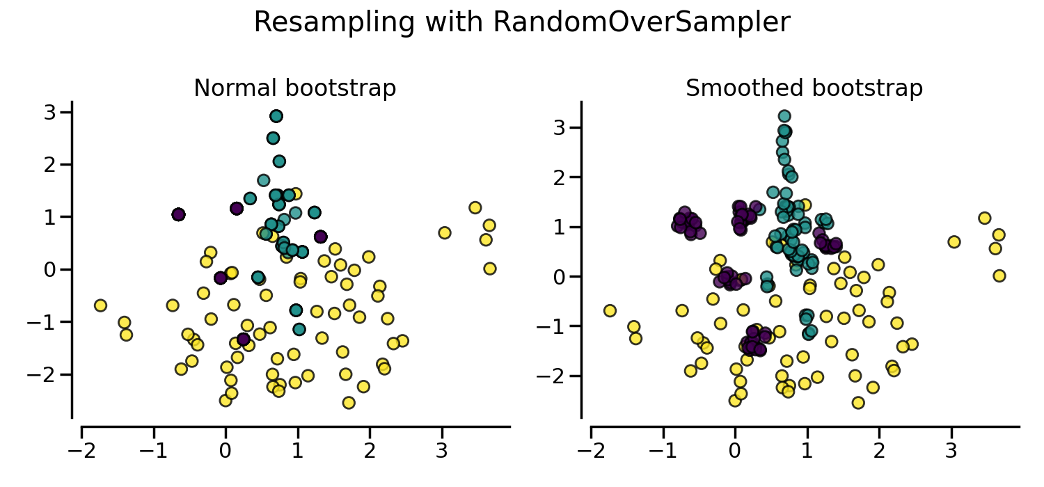
It looks like more samples are generated with smoothed bootstrap. This is due to the fact that the samples generated are not superimposing with the original samples.

More advanced over-sampling using ADASYN and SMOTE

Instead of repeating the same samples when over-sampling or perturbating the generated bootstrap samples, one can use some specific heuristic instead. ADASYN and SMOTE can be used in this case.

from imblearn import FunctionSampler  # to use a idendity sampler
from imblearn.over_sampling import ADASYN, SMOTE

X, y = create_dataset(n_samples=150, weights=(0.1, 0.2, 0.7))

fig, axs = plt.subplots(nrows=2, ncols=2, figsize=(15, 15))

samplers = [
    FunctionSampler(),
    RandomOverSampler(random_state=0),
    SMOTE(random_state=0),
    ADASYN(random_state=0),
]

for ax, sampler in zip(axs.ravel(), samplers):
    title = "Original dataset" if isinstance(sampler, FunctionSampler) else None
    plot_resampling(X, y, sampler, ax, title=title)
fig.tight_layout()

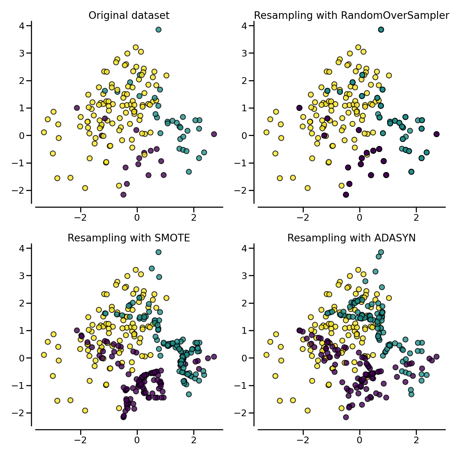
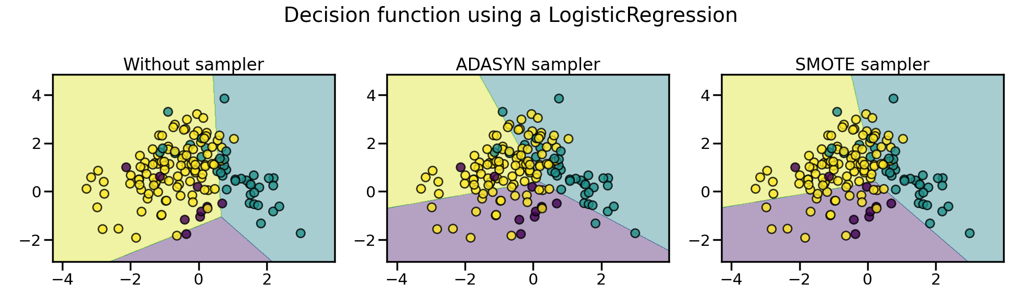
The following plot illustrates the difference between ADASYN and SMOTE. ADASYN will focus on the samples which are difficult to classify with a nearest-neighbors rule while regular SMOTE will not make any distinction. Therefore, the decision function depending of the algorithm.

X, y = create_dataset(n_samples=150, weights=(0.05, 0.25, 0.7))

fig, axs = plt.subplots(nrows=1, ncols=3, figsize=(20, 6))

models = {
    "Without sampler": clf,
    "ADASYN sampler": make_pipeline(ADASYN(random_state=0), clf),
    "SMOTE sampler": make_pipeline(SMOTE(random_state=0), clf),
}

for ax, (title, model) in zip(axs, models.items()):
    model.fit(X, y)
    plot_decision_function(X, y, model, ax=ax, title=title)

fig.suptitle(f"Decision function using a {clf.__class__.__name__}")
fig.tight_layout()

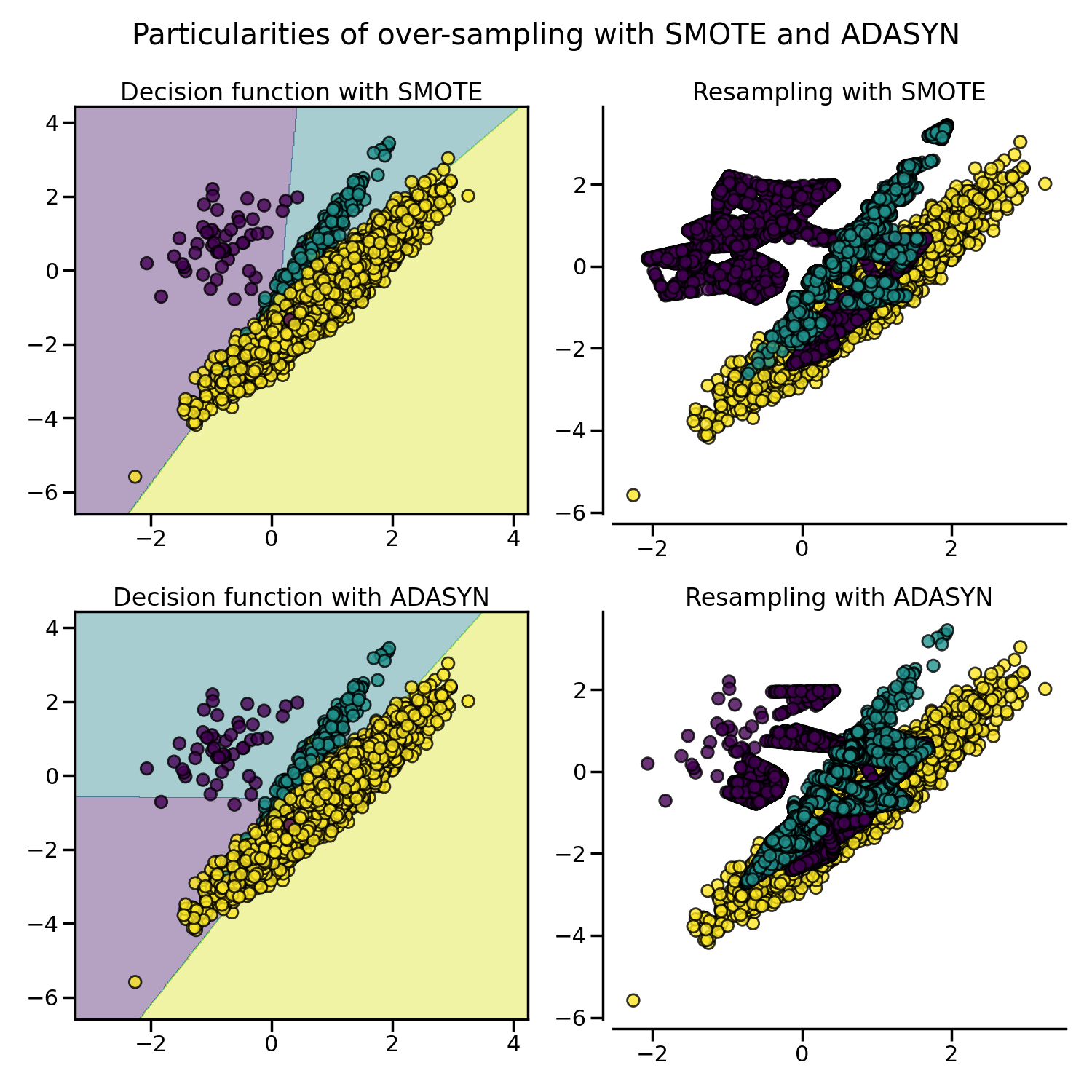
Due to those sampling particularities, it can give rise to some specific issues as illustrated below.

X, y = create_dataset(n_samples=5000, weights=(0.01, 0.05, 0.94), class_sep=0.8)

samplers = [SMOTE(random_state=0), ADASYN(random_state=0)]

fig, axs = plt.subplots(nrows=2, ncols=2, figsize=(15, 15))
for ax, sampler in zip(axs, samplers):
    model = make_pipeline(sampler, clf).fit(X, y)
    plot_decision_function(
        X, y, clf, ax[0], title=f"Decision function with {sampler.__class__.__name__}"
    )
    plot_resampling(X, y, sampler, ax[1])

fig.suptitle("Particularities of over-sampling with SMOTE and ADASYN")
fig.tight_layout()

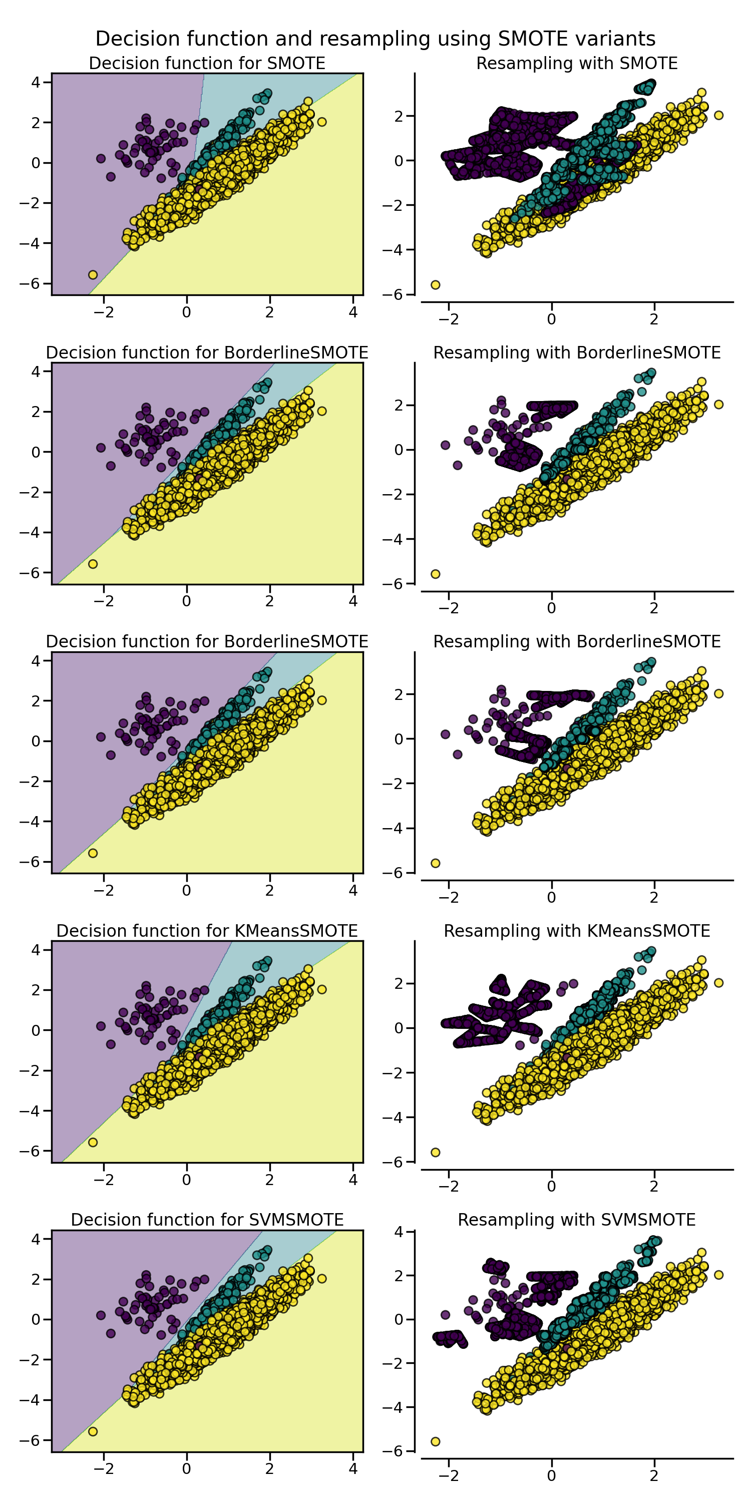
SMOTE proposes several variants by identifying specific samples to consider during the resampling. The borderline version (BorderlineSMOTE) will detect which point to select which are in the border between two classes. The SVM version (SVMSMOTE) will use the support vectors found using an SVM algorithm to create new sample while the KMeans version (KMeansSMOTE) will make a clustering before to generate samples in each cluster independently depending each cluster density.

from sklearn.cluster import MiniBatchKMeans

from imblearn.over_sampling import SVMSMOTE, BorderlineSMOTE, KMeansSMOTE

X, y = create_dataset(n_samples=5000, weights=(0.01, 0.05, 0.94), class_sep=0.8)

fig, axs = plt.subplots(5, 2, figsize=(15, 30))

samplers = [
    SMOTE(random_state=0),
    BorderlineSMOTE(random_state=0, kind="borderline-1"),
    BorderlineSMOTE(random_state=0, kind="borderline-2"),
    KMeansSMOTE(
        kmeans_estimator=MiniBatchKMeans(n_clusters=10, n_init=1, random_state=0),
        random_state=0,
    ),
    SVMSMOTE(random_state=0),
]

for ax, sampler in zip(axs, samplers):
    model = make_pipeline(sampler, clf).fit(X, y)
    plot_decision_function(
        X, y, clf, ax[0], title=f"Decision function for {sampler.__class__.__name__}"
    )
    plot_resampling(X, y, sampler, ax[1])

fig.suptitle("Decision function and resampling using SMOTE variants")
fig.tight_layout()

When dealing with a mixed of continuous and categorical features, SMOTENC is the only method which can handle this case.

from collections import Counter

from imblearn.over_sampling import SMOTENC

rng = np.random.RandomState(42)
n_samples = 50
# Create a dataset of a mix of numerical and categorical data
X = np.empty((n_samples, 3), dtype=object)
X[:, 0] = rng.choice(["A", "B", "C"], size=n_samples).astype(object)
X[:, 1] = rng.randn(n_samples)
X[:, 2] = rng.randint(3, size=n_samples)
y = np.array([0] * 20 + [1] * 30)

print("The original imbalanced dataset")
print(sorted(Counter(y).items()))
print()
print("The first and last columns are containing categorical features:")
print(X[:5])
print()

smote_nc = SMOTENC(categorical_features=[0, 2], random_state=0)
X_resampled, y_resampled = smote_nc.fit_resample(X, y)
print("Dataset after resampling:")
print(sorted(Counter(y_resampled).items()))
print()
print("SMOTE-NC will generate categories for the categorical features:")
print(X_resampled[-5:])
print()

The original imbalanced dataset
[(0, 20), (1, 30)]

The first and last columns are containing categorical features:
[['C' -0.14021849735700803 2]
 ['A' -0.033193400066544886 2]
 ['C' -0.7490765234433554 1]
 ['C' -0.7783820070908942 2]
 ['A' 0.948842857719016 2]]

Dataset after resampling:
[(0, 30), (1, 30)]

SMOTE-NC will generate categories for the categorical features:
[['A' 0.1989993778979113 2]
 ['B' -0.3657680728116921 2]
 ['B' 0.8790828729585258 2]
 ['B' 0.3710891618824609 2]
 ['B' 0.3327240726719727 2]]

However, if the dataset is composed of only categorical features then one should use SMOTEN.

from imblearn.over_sampling import SMOTEN

# Generate only categorical data
X = np.array(["A"] * 10 + ["B"] * 20 + ["C"] * 30, dtype=object).reshape(-1, 1)
y = np.array([0] * 20 + [1] * 40, dtype=np.int32)

print(f"Original class counts: {Counter(y)}")
print()
print(X[:5])
print()

sampler = SMOTEN(random_state=0)
X_res, y_res = sampler.fit_resample(X, y)
print(f"Class counts after resampling {Counter(y_res)}")
print()
print(X_res[-5:])
print()

Original class counts: Counter({1: 40, 0: 20})

[['A']
 ['A']
 ['A']
 ['A']
 ['A']]

Class counts after resampling Counter({0: 40, 1: 40})

[['B']
 ['B']
 ['A']
 ['B']
 ['A']]

Estimated memory usage: 321 MB