Note
Go to the end to download the full example code.
Compare ensemble classifiers using resampling#
Ensemble classifiers have shown to improve classification performance compare to single learner. However, they will be affected by class imbalance. This example shows the benefit of balancing the training set before to learn learners. We are making the comparison with non-balanced ensemble methods.
We make a comparison using the balanced accuracy and geometric mean which are metrics widely used in the literature to evaluate models learned on imbalanced set.
# Authors: Guillaume Lemaitre <g.lemaitre58@gmail.com>
# License: MIT
print(__doc__)
Load an imbalanced dataset#
We will load the UCI SatImage dataset which has an imbalanced ratio of 9.3:1 (number of majority sample for a minority sample). The data are then split into training and testing.
from sklearn.model_selection import train_test_split
from imblearn.datasets import fetch_datasets

satimage = fetch_datasets()["satimage"]
X, y = satimage.data, satimage.target
X_train, X_test, y_train, y_test = train_test_split(X, y, stratify=y, random_state=0)
Classification using a single decision tree#
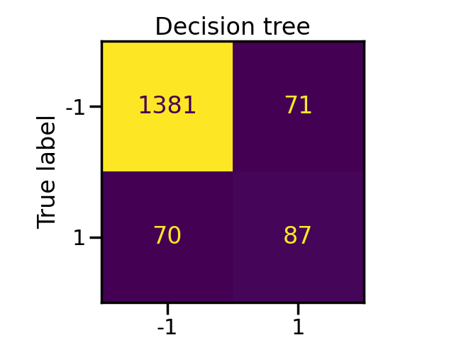
We train a decision tree classifier which will be used as a baseline for the rest of this example.
The results are reported in terms of balanced accuracy and geometric mean which are metrics widely used in the literature to validate model trained on imbalanced set.
from sklearn.tree import DecisionTreeClassifier

tree = DecisionTreeClassifier()
tree.fit(X_train, y_train)
y_pred_tree = tree.predict(X_test)
from sklearn.metrics import balanced_accuracy_score

from imblearn.metrics import geometric_mean_score

print("Decision tree classifier performance:")
print(
    f"Balanced accuracy: {balanced_accuracy_score(y_test, y_pred_tree):.2f} - "
    f"Geometric mean {geometric_mean_score(y_test, y_pred_tree):.2f}"
)
Decision tree classifier performance:
Balanced accuracy: 0.76 - Geometric mean 0.74
import seaborn as sns
from sklearn.metrics import ConfusionMatrixDisplay

sns.set_context("poster")

disp = ConfusionMatrixDisplay.from_estimator(tree, X_test, y_test, colorbar=False)
_ = disp.ax_.set_title("Decision tree")

Classification using bagging classifier with and without sampling#
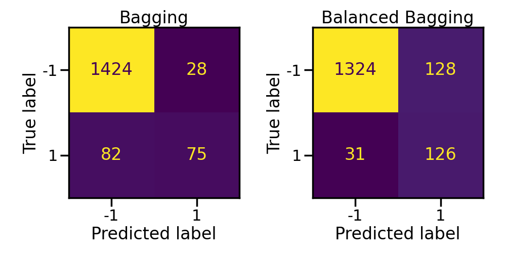
Instead of using a single tree, we will check if an ensemble of decision tree can actually alleviate the issue induced by the class imbalancing. First, we will use a bagging classifier and its counter part which internally uses a random under-sampling to balanced each bootstrap sample.
from sklearn.ensemble import BaggingClassifier

from imblearn.ensemble import BalancedBaggingClassifier

bagging = BaggingClassifier(n_estimators=50, random_state=0)
balanced_bagging = BalancedBaggingClassifier(n_estimators=50, random_state=0)

bagging.fit(X_train, y_train)
balanced_bagging.fit(X_train, y_train)

y_pred_bc = bagging.predict(X_test)
y_pred_bbc = balanced_bagging.predict(X_test)
Balancing each bootstrap sample allows to increase significantly the balanced accuracy and the geometric mean.
print("Bagging classifier performance:")
print(
    f"Balanced accuracy: {balanced_accuracy_score(y_test, y_pred_bc):.2f} - "
    f"Geometric mean {geometric_mean_score(y_test, y_pred_bc):.2f}"
)
print("Balanced Bagging classifier performance:")
print(
    f"Balanced accuracy: {balanced_accuracy_score(y_test, y_pred_bbc):.2f} - "
    f"Geometric mean {geometric_mean_score(y_test, y_pred_bbc):.2f}"
)
Bagging classifier performance:
Balanced accuracy: 0.73 - Geometric mean 0.68
Balanced Bagging classifier performance:
Balanced accuracy: 0.86 - Geometric mean 0.86
import matplotlib.pyplot as plt

fig, axs = plt.subplots(ncols=2, figsize=(10, 5))
ConfusionMatrixDisplay.from_estimator(
    bagging, X_test, y_test, ax=axs[0], colorbar=False
)
axs[0].set_title("Bagging")

ConfusionMatrixDisplay.from_estimator(
    balanced_bagging, X_test, y_test, ax=axs[1], colorbar=False
)
axs[1].set_title("Balanced Bagging")

fig.tight_layout()

Classification using random forest classifier with and without sampling#
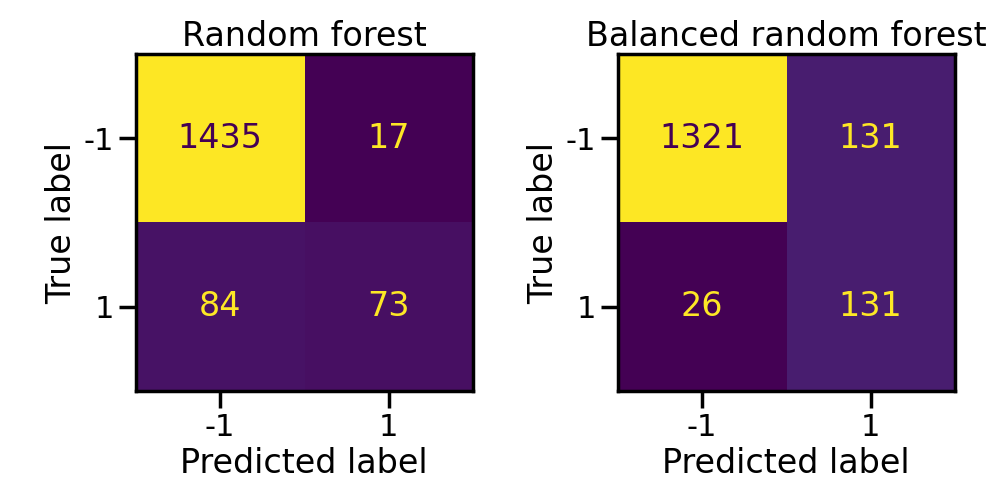
Random forest is another popular ensemble method and it is usually outperforming bagging. Here, we used a vanilla random forest and its balanced counterpart in which each bootstrap sample is balanced.
from sklearn.ensemble import RandomForestClassifier

from imblearn.ensemble import BalancedRandomForestClassifier

rf = RandomForestClassifier(n_estimators=50, random_state=0)
brf = BalancedRandomForestClassifier(
    n_estimators=50,
    sampling_strategy="all",
    replacement=True,
    bootstrap=False,
    random_state=0,
)

rf.fit(X_train, y_train)
brf.fit(X_train, y_train)

y_pred_rf = rf.predict(X_test)
y_pred_brf = brf.predict(X_test)
Similarly to the previous experiment, the balanced classifier outperform the classifier which learn from imbalanced bootstrap samples. In addition, random forest outperforms the bagging classifier.
print("Random Forest classifier performance:")
print(
    f"Balanced accuracy: {balanced_accuracy_score(y_test, y_pred_rf):.2f} - "
    f"Geometric mean {geometric_mean_score(y_test, y_pred_rf):.2f}"
)
print("Balanced Random Forest classifier performance:")
print(
    f"Balanced accuracy: {balanced_accuracy_score(y_test, y_pred_brf):.2f} - "
    f"Geometric mean {geometric_mean_score(y_test, y_pred_brf):.2f}"
)
Random Forest classifier performance:
Balanced accuracy: 0.73 - Geometric mean 0.68
Balanced Random Forest classifier performance:
Balanced accuracy: 0.87 - Geometric mean 0.87
fig, axs = plt.subplots(ncols=2, figsize=(10, 5))
ConfusionMatrixDisplay.from_estimator(rf, X_test, y_test, ax=axs[0], colorbar=False)
axs[0].set_title("Random forest")

ConfusionMatrixDisplay.from_estimator(brf, X_test, y_test, ax=axs[1], colorbar=False)
axs[1].set_title("Balanced random forest")

fig.tight_layout()

Boosting classifier#
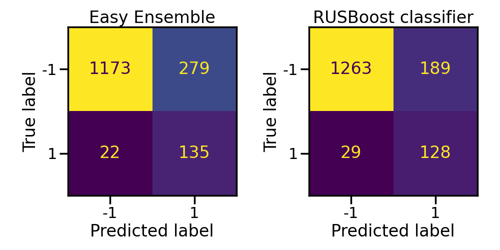
In the same manner, easy ensemble classifier is a bag of balanced AdaBoost classifier. However, it will be slower to train than random forest and will achieve worse performance.
from sklearn.ensemble import AdaBoostClassifier

from imblearn.ensemble import EasyEnsembleClassifier, RUSBoostClassifier

estimator = AdaBoostClassifier(n_estimators=10)
eec = EasyEnsembleClassifier(n_estimators=10, estimator=estimator)
eec.fit(X_train, y_train)
y_pred_eec = eec.predict(X_test)

rusboost = RUSBoostClassifier(n_estimators=10, estimator=estimator)
rusboost.fit(X_train, y_train)
y_pred_rusboost = rusboost.predict(X_test)
print("Easy ensemble classifier performance:")
print(
    f"Balanced accuracy: {balanced_accuracy_score(y_test, y_pred_eec):.2f} - "
    f"Geometric mean {geometric_mean_score(y_test, y_pred_eec):.2f}"
)
print("RUSBoost classifier performance:")
print(
    f"Balanced accuracy: {balanced_accuracy_score(y_test, y_pred_rusboost):.2f} - "
    f"Geometric mean {geometric_mean_score(y_test, y_pred_rusboost):.2f}"
)
Easy ensemble classifier performance:
Balanced accuracy: 0.83 - Geometric mean 0.83
RUSBoost classifier performance:
Balanced accuracy: 0.82 - Geometric mean 0.82
fig, axs = plt.subplots(ncols=2, figsize=(10, 5))

ConfusionMatrixDisplay.from_estimator(eec, X_test, y_test, ax=axs[0], colorbar=False)
axs[0].set_title("Easy Ensemble")
ConfusionMatrixDisplay.from_estimator(
    rusboost, X_test, y_test, ax=axs[1], colorbar=False
)
axs[1].set_title("RUSBoost classifier")

fig.tight_layout()
plt.show()

Total running time of the script: (0 minutes 44.767 seconds)
Estimated memory usage: 436 MB

