Effect of the shrinkage factor in random over-sampling

This example shows the effect of the shrinkage factor used to generate the smoothed bootstrap using the RandomOverSampler.

# Authors: Guillaume Lemaitre <g.lemaitre58@gmail.com>
# License: MIT

print(__doc__)

import seaborn as sns

sns.set_context("poster")

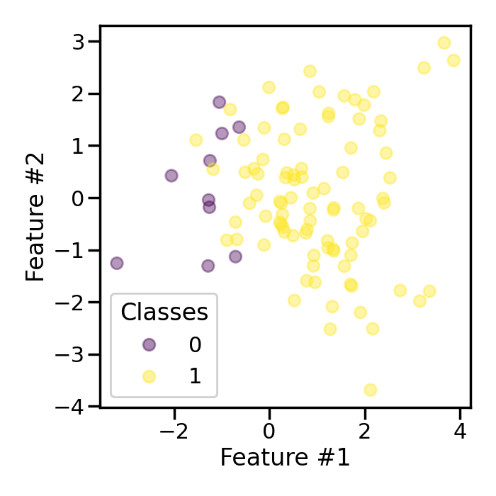
First, we will generate a toy classification dataset with only few samples. The ratio between the classes will be imbalanced.

from collections import Counter

from sklearn.datasets import make_classification

X, y = make_classification(
    n_samples=100,
    n_features=2,
    n_redundant=0,
    weights=[0.1, 0.9],
    random_state=0,
)
Counter(y)

Counter({1: 90, 0: 10})

import matplotlib.pyplot as plt

fig, ax = plt.subplots(figsize=(7, 7))
scatter = plt.scatter(X[:, 0], X[:, 1], c=y, alpha=0.4)
class_legend = ax.legend(*scatter.legend_elements(), loc="lower left", title="Classes")
ax.add_artist(class_legend)
ax.set_xlabel("Feature #1")
_ = ax.set_ylabel("Feature #2")
plt.tight_layout()

Now, we will use a RandomOverSampler to generate a bootstrap for the minority class with as many samples as in the majority class.

from imblearn.over_sampling import RandomOverSampler

sampler = RandomOverSampler(random_state=0)
X_res, y_res = sampler.fit_resample(X, y)
Counter(y_res)

Counter({1: 90, 0: 90})

fig, ax = plt.subplots(figsize=(7, 7))
scatter = plt.scatter(X_res[:, 0], X_res[:, 1], c=y_res, alpha=0.4)
class_legend = ax.legend(*scatter.legend_elements(), loc="lower left", title="Classes")
ax.add_artist(class_legend)
ax.set_xlabel("Feature #1")
_ = ax.set_ylabel("Feature #2")
plt.tight_layout()

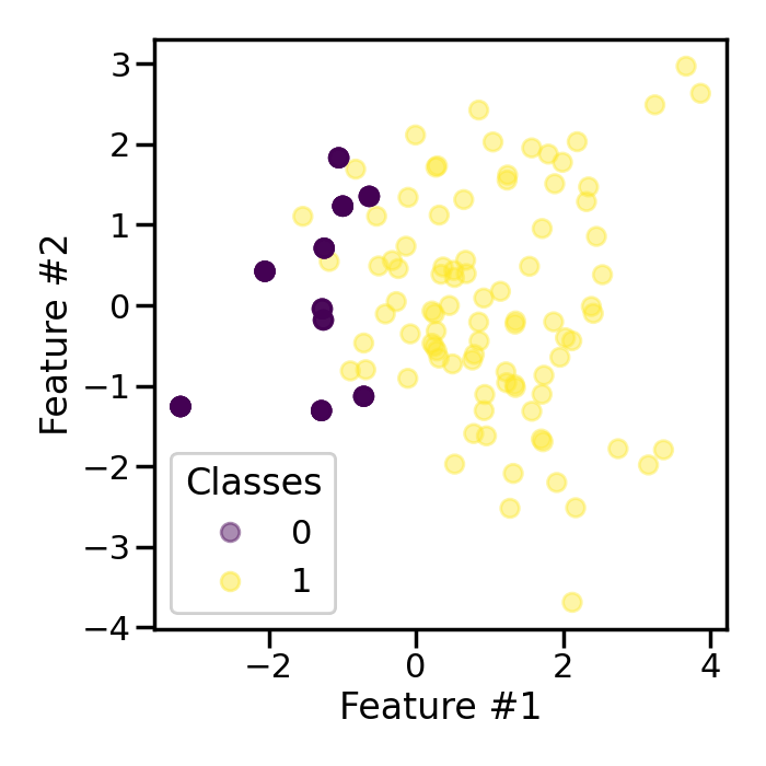
We observe that the minority samples are less transparent than the samples from the majority class. Indeed, it is due to the fact that these samples of the minority class are repeated during the bootstrap generation.

We can set shrinkage to a floating value to add a small perturbation to the samples created and therefore create a smoothed bootstrap.

sampler = RandomOverSampler(shrinkage=1, random_state=0)
X_res, y_res = sampler.fit_resample(X, y)
Counter(y_res)

Counter({1: 90, 0: 90})

fig, ax = plt.subplots(figsize=(7, 7))
scatter = plt.scatter(X_res[:, 0], X_res[:, 1], c=y_res, alpha=0.4)
class_legend = ax.legend(*scatter.legend_elements(), loc="lower left", title="Classes")
ax.add_artist(class_legend)
ax.set_xlabel("Feature #1")
_ = ax.set_ylabel("Feature #2")
plt.tight_layout()

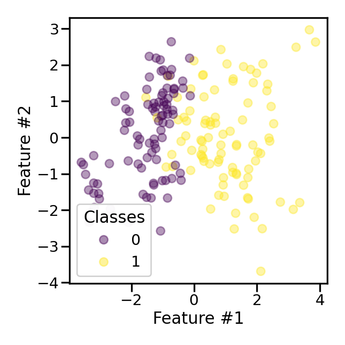
In this case, we see that the samples in the minority class are not overlapping anymore due to the added noise.

The parameter shrinkage allows to add more or less perturbation. Let’s add more perturbation when generating the smoothed bootstrap.

sampler = RandomOverSampler(shrinkage=3, random_state=0)
X_res, y_res = sampler.fit_resample(X, y)
Counter(y_res)

Counter({1: 90, 0: 90})

fig, ax = plt.subplots(figsize=(7, 7))
scatter = plt.scatter(X_res[:, 0], X_res[:, 1], c=y_res, alpha=0.4)
class_legend = ax.legend(*scatter.legend_elements(), loc="lower left", title="Classes")
ax.add_artist(class_legend)
ax.set_xlabel("Feature #1")
_ = ax.set_ylabel("Feature #2")
plt.tight_layout()

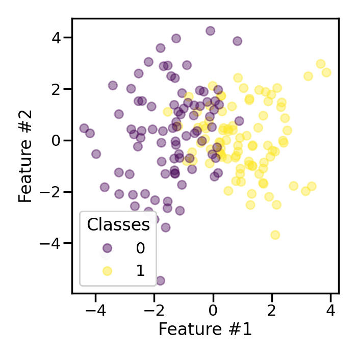
Increasing the value of shrinkage will disperse the new samples. Forcing the shrinkage to 0 will be equivalent to generating a normal bootstrap.

sampler = RandomOverSampler(shrinkage=0, random_state=0)
X_res, y_res = sampler.fit_resample(X, y)
Counter(y_res)

Counter({1: 90, 0: 90})

fig, ax = plt.subplots(figsize=(7, 7))
scatter = plt.scatter(X_res[:, 0], X_res[:, 1], c=y_res, alpha=0.4)
class_legend = ax.legend(*scatter.legend_elements(), loc="lower left", title="Classes")
ax.add_artist(class_legend)
ax.set_xlabel("Feature #1")
_ = ax.set_ylabel("Feature #2")
plt.tight_layout()

Therefore, the shrinkage is handy to manually tune the dispersion of the new samples.

Estimated memory usage: 10 MB