Compare sampler combining over- and under-sampling

This example shows the effect of applying an under-sampling algorithms after SMOTE over-sampling. In the literature, Tomek’s link and edited nearest neighbours are the two methods which have been used and are available in imbalanced-learn.

# Authors: Guillaume Lemaitre <g.lemaitre58@gmail.com>
# License: MIT

print(__doc__)

import matplotlib.pyplot as plt
import seaborn as sns

sns.set_context("poster")

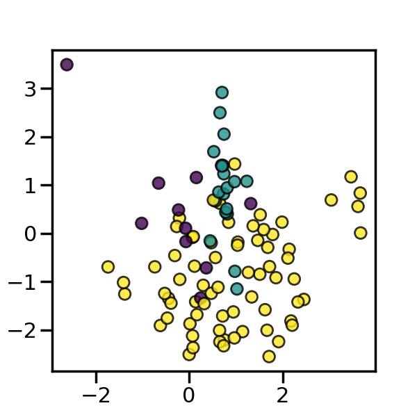
Dataset generation

We will create an imbalanced dataset with a couple of samples. We will use make_classification to generate this dataset.

from sklearn.datasets import make_classification

X, y = make_classification(
    n_samples=100,
    n_features=2,
    n_informative=2,
    n_redundant=0,
    n_repeated=0,
    n_classes=3,
    n_clusters_per_class=1,
    weights=[0.1, 0.2, 0.7],
    class_sep=0.8,
    random_state=0,
)

_, ax = plt.subplots(figsize=(6, 6))
_ = ax.scatter(X[:, 0], X[:, 1], c=y, alpha=0.8, edgecolor="k")

The following function will be used to plot the sample space after resampling to illustrate the characteristic of an algorithm.

from collections import Counter


def plot_resampling(X, y, sampler, ax):
    """Plot the resampled dataset using the sampler."""
    X_res, y_res = sampler.fit_resample(X, y)
    ax.scatter(X_res[:, 0], X_res[:, 1], c=y_res, alpha=0.8, edgecolor="k")
    sns.despine(ax=ax, offset=10)
    ax.set_title(f"Decision function for {sampler.__class__.__name__}")
    return Counter(y_res)

The following function will be used to plot the decision function of a classifier given some data.

import numpy as np


def plot_decision_function(X, y, clf, ax):
    """Plot the decision function of the classifier and the original data"""
    plot_step = 0.02
    x_min, x_max = X[:, 0].min() - 1, X[:, 0].max() + 1
    y_min, y_max = X[:, 1].min() - 1, X[:, 1].max() + 1
    xx, yy = np.meshgrid(
        np.arange(x_min, x_max, plot_step), np.arange(y_min, y_max, plot_step)
    )

    Z = clf.predict(np.c_[xx.ravel(), yy.ravel()])
    Z = Z.reshape(xx.shape)
    ax.contourf(xx, yy, Z, alpha=0.4)
    ax.scatter(X[:, 0], X[:, 1], alpha=0.8, c=y, edgecolor="k")
    ax.set_title(f"Resampling using {clf[0].__class__.__name__}")

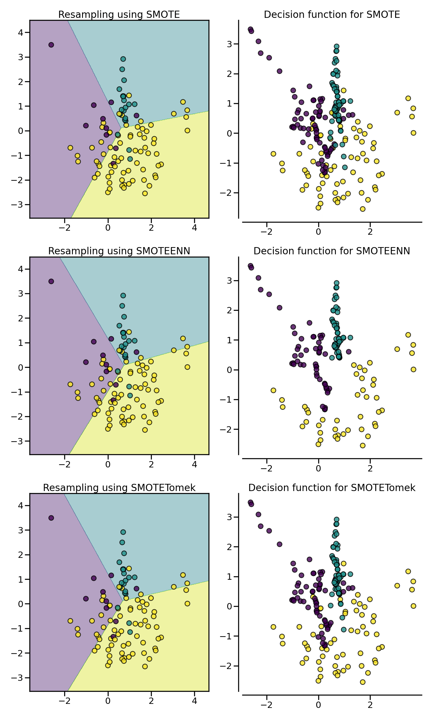
SMOTE allows to generate samples. However, this method of over-sampling does not have any knowledge regarding the underlying distribution. Therefore, some noisy samples can be generated, e.g. when the different classes cannot be well separated. Hence, it can be beneficial to apply an under-sampling algorithm to clean the noisy samples. Two methods are usually used in the literature: (i) Tomek’s link and (ii) edited nearest neighbours cleaning methods. Imbalanced-learn provides two ready-to-use samplers SMOTETomek and SMOTEENN. In general, SMOTEENN cleans more noisy data than SMOTETomek.

from sklearn.linear_model import LogisticRegression

from imblearn.combine import SMOTEENN, SMOTETomek

from imblearn.over_sampling import SMOTE
from imblearn.pipeline import make_pipeline

samplers = [SMOTE(random_state=0), SMOTEENN(random_state=0), SMOTETomek(random_state=0)]

fig, axs = plt.subplots(3, 2, figsize=(15, 25))
for ax, sampler in zip(axs, samplers):
    clf = make_pipeline(sampler, LogisticRegression()).fit(X, y)
    plot_decision_function(X, y, clf, ax[0])
    plot_resampling(X, y, sampler, ax[1])
fig.tight_layout()

plt.show()

Estimated memory usage: 213 MB