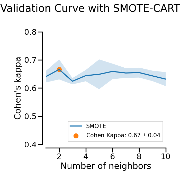
Plotting Validation Curves

In this example the impact of the SMOTE’s k_neighbors parameter is examined. In the plot you can see the validation scores of a SMOTE-CART classifier for different values of the SMOTE’s k_neighbors parameter.

# Authors: Christos Aridas
#          Guillaume Lemaitre <g.lemaitre58@gmail.com>
# License: MIT

print(__doc__)

import seaborn as sns

sns.set_context("poster")


RANDOM_STATE = 42

Let’s first generate a dataset with imbalanced class distribution.

from sklearn.datasets import make_classification

X, y = make_classification(
    n_classes=2,
    class_sep=2,
    weights=[0.1, 0.9],
    n_informative=10,
    n_redundant=1,
    flip_y=0,
    n_features=20,
    n_clusters_per_class=4,
    n_samples=5000,
    random_state=RANDOM_STATE,
)

We will use an over-sampler SMOTE followed by a DecisionTreeClassifier. The aim will be to search which k_neighbors parameter is the most adequate with the dataset that we generated.

from sklearn.tree import DecisionTreeClassifier

from imblearn.over_sampling import SMOTE
from imblearn.pipeline import make_pipeline

model = make_pipeline(
    SMOTE(random_state=RANDOM_STATE), DecisionTreeClassifier(random_state=RANDOM_STATE)
)

We can use the validation_curve to inspect the impact of varying the parameter k_neighbors. In this case, we need to use a score to evaluate the generalization score during the cross-validation.

from sklearn.metrics import cohen_kappa_score, make_scorer
from sklearn.model_selection import validation_curve

scorer = make_scorer(cohen_kappa_score)
param_range = range(1, 11)
train_scores, test_scores = validation_curve(
    model,
    X,
    y,
    param_name="smote__k_neighbors",
    param_range=param_range,
    cv=3,
    scoring=scorer,
)

train_scores_mean = train_scores.mean(axis=1)
train_scores_std = train_scores.std(axis=1)
test_scores_mean = test_scores.mean(axis=1)
test_scores_std = test_scores.std(axis=1)

We can now plot the results of the cross-validation for the different parameter values that we tried.

import matplotlib.pyplot as plt

fig, ax = plt.subplots(figsize=(7, 7))
ax.plot(param_range, test_scores_mean, label="SMOTE")
ax.fill_between(
    param_range,
    test_scores_mean + test_scores_std,
    test_scores_mean - test_scores_std,
    alpha=0.2,
)
idx_max = test_scores_mean.argmax()
ax.scatter(
    param_range[idx_max],
    test_scores_mean[idx_max],
    label=r"Cohen Kappa: ${:.2f}\pm{:.2f}$".format(
        test_scores_mean[idx_max], test_scores_std[idx_max]
    ),
)

fig.suptitle("Validation Curve with SMOTE-CART")
ax.set_xlabel("Number of neighbors")
ax.set_ylabel("Cohen's kappa")

# make nice plotting
sns.despine(ax=ax, offset=10)
ax.set_xlim([1, 10])
ax.set_ylim([0.4, 0.8])
ax.legend(loc="lower right", fontsize=16)
plt.tight_layout()
plt.show()

Estimated memory usage: 10 MB